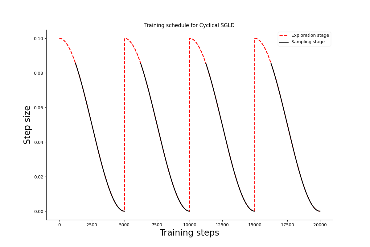
Cyclical schedule

from typing import NamedTuple
 
class ScheduleState(NamedTuple):
    step_size: float
    do_sample: bool
 
def build_schedule(
    num_training_steps,
    num_cycles=4,
    initial_step_size=1e-3,
    exploration_ratio=0.25,
):
    cycle_length = num_training_steps // num_cycles
 
    def schedule_fn(step_id):
        do_sample = False
        if ((step_id % cycle_length)/cycle_length) >= exploration_ratio:
            do_sample = True
 
        cos_out = jnp.cos(jnp.pi * (step_id % cycle_length) / cycle_length) + 1
        step_size = 0.5 * cos_out * initial_step_size
 
        return ScheduleState(step_size, do_sample)
 
    return schedule_fn

Let us visualize the schedule for 200k training steps divided in 4 cycles. At each cycle 1/4th of the steps are dedicated to exploration.

Cyclical SGLD step

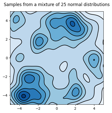
We will reproduce one of the paper’s example, sampling from an array of 25 gaussians.

import itertools
 
import jax
import jax.scipy as jsp
import jax.numpy as jnp
 
lmbda = 1/25
positions = [-4, -2, 0, 2, 4]
mu = jnp.array([list(prod) for prod in itertools.product(positions, positions)])
sigma = 0.03 * jnp.eye(2)
 
def logprob_fn(x, *_):
    return lmbda * jsp.special.logsumexp(
        jax.scipy.stats.multivariate_normal.logpdf(x, mu, sigma)
    )
 
def sample_fn(rng_key):
    choose_key, sample_key = jax.random.split(rng_key)
    samples = jax.random.multivariate_normal(sample_key, mu, sigma)
    return jax.random.choice(choose_key, samples)

Let’s plot the model’s density; we will need the plot later to evaluate the sampler

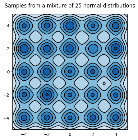
Sample from the mixture of gaussians

The sampling kernel must be able to alternate between sampling and optimization periods that are determined by the scheduler.

from typing import NamedTuple
 
import blackjax
import optax
 
from blackjax.types import PyTree
from optax._src.base import OptState
 
class CyclicalSGMCMCState(NamedTuple):
    """State of the Cyclical SGMCMC sampler."""
    position: PyTree
    opt_state: OptState
 
def cyclical_sgld(grad_estimator_fn, loglikelihood_fn):
 
    sgld = blackjax.sgld(grad_estimator_fn)
    sgd = optax.sgd(1.)
 
    def init_fn(position):
        """Initialize Cyclical SGLD's state."""
        opt_state = sgd.init(position)
        return CyclicalSGMCMCState(position, opt_state)
 
    def step_fn(
        rng_key,
        schedule_state: ScheduleState,
        state: CyclicalSGMCMCState,
        minibatch: PyTree
    ):
        """Cyclical SGLD kernel.
 
        TODO: Organize the inputs to match the SGLD API better.
 
        rng_key
            Key for JAX's pseudo-random number generator.
        schedule_state
            The current state of the scheduler. Indicates whether the kernel
            should be sampling or optimizing, and the current step size.
        state
            The current state of the Cyclical SGLD sampler.
        minibatch
            Not used in the mixture example, but this is where you would pass
            batches of data in any real application.
 
        """
 
        def step_with_sgld(current_state):
            rng_key, state, minibatch, step_size = current_state
            new_position = sgld(rng_key, state.position, minibatch, step_size)
            return CyclicalSGMCMCState(new_position, state.opt_state)
 
        def step_with_sgd(current_state):
            _, state, minibatch, step_size = current_state
            grads = grad_estimator_fn(state.position, minibatch)
            rescaled_grads = - 1. * step_size * grads
            updates, new_opt_state = sgd.update(rescaled_grads, state.opt_state, state.position)
            new_position = optax.apply_updates(state.position, updates)
            return CyclicalSGMCMCState(new_position, new_opt_state)
 
        new_state = jax.lax.cond(
            schedule_state.do_sample,
            step_with_sgld,
            step_with_sgd,
            (rng_key, state, minibatch, schedule_state.step_size)
        )
 
        return new_state
 
    return init_fn, step_fn

SGLD

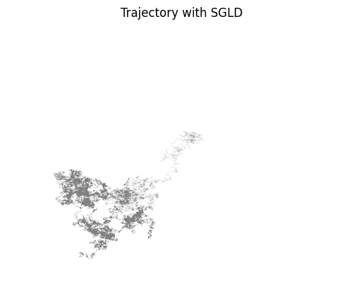
Let’s start with SGLD:

import jax
from fastprogress import progress_bar
 
# 50k iterations
num_training_steps = 50000
schedule_fn = lambda k: 0.05 * k ** (-0.55)
# TODO: There is no need to pre-compute the schedule
schedule = [schedule_fn(i) for i in range(1, num_training_steps+1)]
 
grad_fn = lambda x, _: jax.grad(logprob_fn)(x)
sgld = blackjax.sgld(grad_fn)
 
rng_key = jax.random.PRNGKey(3)
init_position = -10 + 20 * jax.random.uniform(rng_key, shape=(2,))
 
position = init_position
sgld_samples = []
for i in progress_bar(range(num_training_steps)):
    _, rng_key = jax.random.split(rng_key)
    position = jax.jit(sgld)(rng_key, position, 0, schedule[i])
    sgld_samples.append(position)

Let’s plot the trajectory:

Cyclical SGLD

Now let’s sample using Cyclical SGLD.

import jax
from fastprogress import progress_bar
 
# 50k iterations
# M = 30
# initial step size = 0.09
# ratio exploration = 1/4
num_training_steps = 50000
schedule_fn = build_schedule(num_training_steps, 30, 0.09, 0.25)
# TODO: There is no need to pre-compute the schedule
schedule = [schedule_fn(i) for i in range(num_training_steps)]
 
grad_fn = lambda x, _: jax.grad(logprob_fn)(x)
init, step = cyclical_sgld(grad_fn, logprob_fn)
 
rng_key = jax.random.PRNGKey(3)
init_position = -10 + 20 * jax.random.uniform(rng_key, shape=(2,))
init_state = init(init_position)
 
state = init_state
cyclical_samples = []
for i in progress_bar(range(num_training_steps)):
    _, rng_key = jax.random.split(rng_key)
    state = jax.jit(step)(rng_key, schedule[i], state, 0)
    if schedule[i].do_sample:
        cyclical_samples.append(state.position)

It looks from the trajectory that the distribution is better explored:

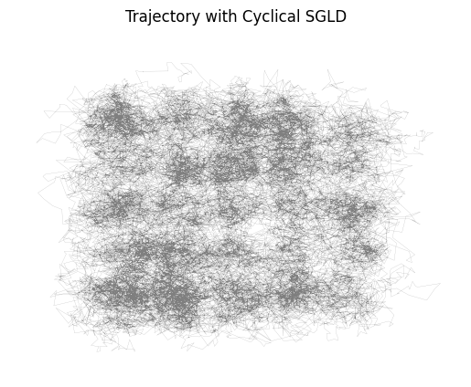
Let’s look at the distribution:

What’s next

As Adrien Corenflos noted, Scott’s rule for KDE assumes that the total number of points is the sample size, so is not fit for MCMC samples. We should instead pass the bandwidth manually $n_{e ff}^{(- 1/ (d + 4))}$ with $d = 2$ ; It should capture more modes.
Compute the paper’s Mode-coverage metric: when the number of samples falling within the radius $r$ of a mode center is larger than a number $N$ when we say the mode is covered;
Use on a “real” problem: CIFAR-100 with Resnet18 for instance;